Time Series

A time series is made of discreet measurements at timed intervals. The time series pattern is a write optimization pattern made to ensure maximum write performance throughput for a typical analytics application that stores data in discrete units of time. Examples can include counting the number of page views in a second, or the temperature per minute. For this schema, we will discuss time series in the context of web page views.

Schema Observations

• The Time series schema is based on efficient, in place updates, which map well to the way the MMAP storage engine works. However, this is not as efficient when using the WiredTiger storage engine due to its lack of in place update support.

Schema

Schema Attributes	Description
Optimized For	Write Performance
Preallocation	Benefits from Preallocation on MMAP

To maximize our write throughput for a time series, we are making the assumptions that we’re interested in discreet buckets of time. That is to say, an individual page view is not attractive to the application by itself. Only the number of page views, in a particular second, minute, hour, day or in a date and time range are of interest. This means the smallest unit of time we want for this example, is a single minute.

Taking that into account, let’s model a bucket to keep all our page views for a particular minute.

{
  "page": "/index.htm",
  "timestamp": ISODate("2014-01-01T10:01:00Z"),
  "totalViews": 0,
  "seconds": {
    "0": 0
  }
}

Example 1: A time series bucket

Breaking down the fields.

Schema Attributes	Description
page	The web page we are measuring
timestamp	The actual minute the bucket is for
totalViews	Total page views in this minute
seconds	Page views for a specific second in the minute

The bucket document not only represents the complete number of page views in a particular minute but also contains the breakdown of page views per second inside that minute.

Operations

Update the Page Views in a Bucket

Let’s simulate what happens in an application that is counting page views for a specific page. We are going to simulate updating a bucket, for a specific page view in the 2nd second of the ISODate("2014-01-01T10:01:00Z") bucket.

var col = db.getSisterDB("timeseries").pageViews;
var secondInMinute = 2;
var updateStatment = {$inc: {}};
updateStatment["$inc"]["seconds." + secondInMinute] = 1;

col.update({
  page: "/index.htm",
  timestamp: ISODate("2014-01-01T10:01:00Z")
}, updateStatment, true)

Example 2: Updating a bucket

The first part of the updateStatement sets up the $inc value to increment the field in the seconds field named 2, which corresponds with the secondary elapsed second in our bucket time period.

If the field does not exist MongoDB, will set it to one. Otherwise, it will increment the existing value with one. Notice the last parameter of the update statement. This is telling MongoDB to do an upsert which instructs MongoDB to create a new document if none exists that matches the update selector.

Retrieving a specific Bucket

If we wish to retrieve a specific time measurement bucket for a particular minute, we can retrieve it very easily using the timestamp field as shown below.

var col = db.getSisterDB("timeseries").pageViews;
pageViews.findOne({
  page: "/index.htm",
  timestamp: ISODate("2014-01-01T10:01:00Z")
});

Example 3: Retrieve a specific bucket

This will retrieve the bucket for which the timestamp matches the time bucket ISODate("2014-01-01T10:01:00Z").

Pre-allocating measurement buckets

To improve performance on writes, we can preallocate buckets to avoid the need to move documents around in memory and on disk. Each bucket document has a known fixed final size. If we use a template to create the empty buckets, we can take advantage of in place updates, minimizing the amount of disk IO needed to collect the page views.

Let’s look at how we can preallocate buckets for a whole hour of measurements. The example function below preAllocateHour, takes a collection, a web page name and a timestamp representing a specific hour.

var preAllocateHour = function(coll, pageName, timestamp) {
  for(var i = 0; i < 60; i++) {
    coll.insert({
      "page": pageName,
      "timestamp" : timestamp,
      "seconds" : {
        "0":0,"1":0,"2":0,"3":0,"4":0,"5":0,"6":0,"7":0,"8":0,"9":0,
        "10":0,"11":0,"12":0,"13":0,"14":0,"15":0,"16":0,"17":0,"18":0,"19":0,
        "20":0,"21":0,"22":0,"23":0,"24":0,"25":0,"26":0,"27":0,"28":0,"29":0,
        "30":0,"31":0,"32":0,"33":0,"34":0,"35":0,"36":0,"37":0,"38":0,"39":0,
        "40":0,"41":0,"42":0,"43":0,"44":0,"45":0,"46":0,"47":0,"48":0,"49":0,
        "50":0,"51":0,"52":0,"53":0,"54":0,"55":0,"56":0,"57":0,"58":0,"59":0
      }
    })

    timestamp.setMinutes(timestamp.getMinutes() + 1);
  }
}

Example 4: Pre-Allocate buckets for a specific hour

Let’s take this preallocation method out for a test run by preallocating an hour worth of buckets.

var col = db.getSisterDB("analytics").pageViews;
preAllocateHour(col, "index.htm", ISODate("2014-01-01T10:00:00Z"));

Example 5: Call the preAllocate method for a specific hour

Let’s verify that the preallocation of buckets happened correctly by counting the number of bucket entries generated for the specific hour.

var col = db.getSisterDB("analytics").pageViews;
col.find({timestamp: {$gte: ISODate("2014-01-01T10:00:00Z")},timestamp: {$lt: ISODate("2014-01-01T11:00:00Z")} }).count()

Example 6: Retrieve the number of documents created by the preAllocateHour method

As we expected the count returned is 60 entries.

Indexes

Since we will be retrieving the timestamp buckets by their page name and timestamp, the only needed indexes for efficiency are on the page and timestamp fields.

var col = db.getSisterDB("timeseries").pageViews;
col.ensureIndex({page:1, timestamp: 1});

Example 7: Create the timestamp index

This will ensure any range queries across the timestamp field will be able to leverage the index for better query performance.

Scaling

Secondary Reads

Secondary reads might be useful when reporting on the data, as any long running reports on them will cause minimal impact to write throughput.

Sharding

Picking a shard key for a time series will impact the way the data is written and the way it’s read.

In the case of the web page analytics example, we wish to summarize the data by page. If the writes for a particular web page are spread out among all the shards, we require scatter/gather queries to correctly summarize data for a specific time period.

We want a shard key that will group all measurements for a specific web page on one specific shard but will spread out the pages across all the shards to maximize write throughput.

We can achieve this by creating a compound shard key which contains the web page name as well as the date.

var admin = db.getSisterDB("admin");
db.runCommand({enableSharding:'timeseries'});
db.runCommand({
    shardCollection: 'timeseries.pageViews'
  , key: {page:1, timestamp:1}
});

Example 8: Compound shard key

The benefit of using this shard key is that we can still aggregate all the values for a specific page on one shard without forcing a scatter-gather query.

Performance

A simple exploration of the performance on a single machine with MongoDb 3.0 shows the difference between MMAP and WiredTiger for a narrow simulation using the schema simulation framework mongodb-schema-simulator.

Scenario

https://github.com/christkv/mongodb-schema-simulator/blob/master/examples/scripts/single_or_replset/timeseries/exercise_time_series.js

MongoDb runs locally on a MacBook Pro Retina 2015 with ssd and 16 gb ram. The simulation runs with the following parameters against a single mongodb instance under osx 10.10 Yosemite.

Parameters	Value
processes	4
poolSize per process	50
type	linear
Resolution in milliseconds	1000
Iterations run	25
Number of users updating timeseries per iteration	1000
Execution strategy	slicetime

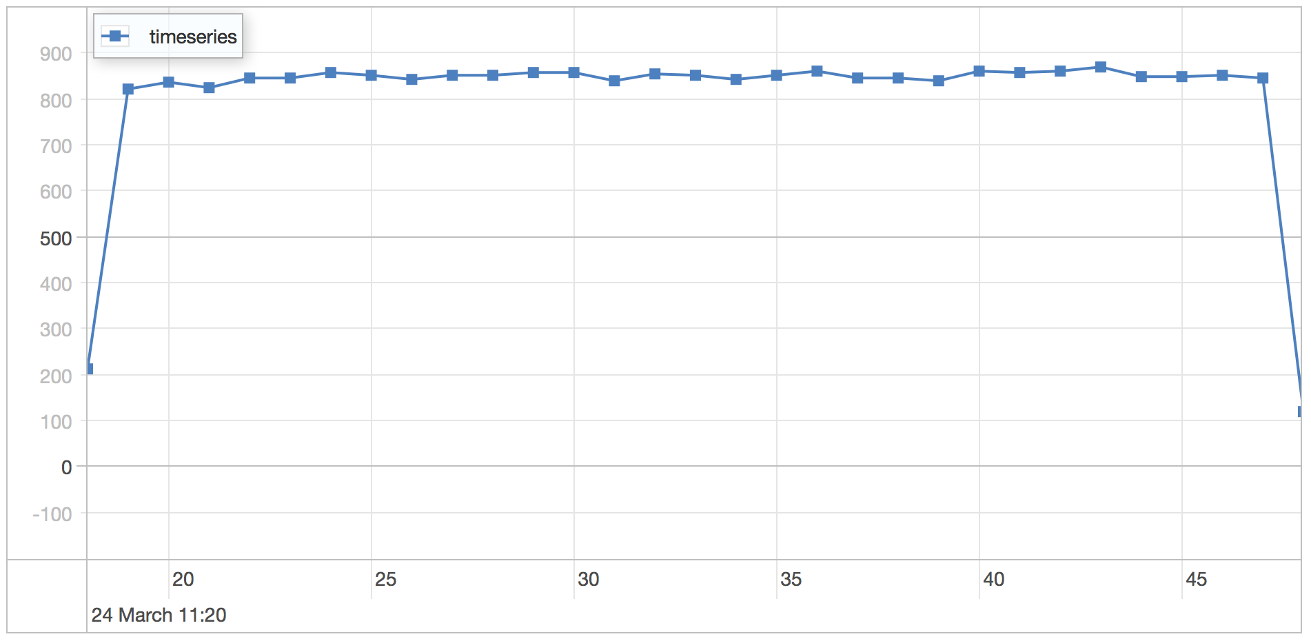
MMAP

The MMAP engine is run using the default settings on MongoDB 3.0.1.

timeseries scenario results

Statistics	Value
Runtime	30.253 seconds
Mean	1.06 milliseconds
Standard Deviation	1.588 milliseconds
75 percentile	1.246 milliseconds
95 percentile	1.502 milliseconds
99 percentile	1.815 milliseconds
Minimum	0.448 milliseconds
Maximum	57.48 milliseconds

Notice that the 2000 users per second impacts the minimum and maximum as well as the average query time quite a bit.

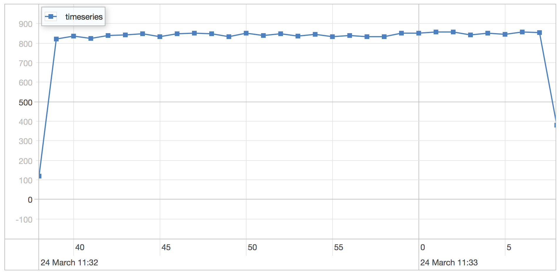
WiredTiger

The WiredTiger engine is run using the default settings on MongoDB 3.0.1.

metadata scenario results

Statistics	Value
Runtime	30.08 seconds
Mean	1.108 milliseconds
Standard Deviation	0.401 milliseconds
75 percentile	1.341 milliseconds
95 percentile	1.871 milliseconds
99 percentile	2.477 milliseconds
Minimum	0.513 milliseconds
Maximum	5.481 milliseconds

As expected there is not much difference between the MMAP and WiredTiger storage engines when it’s a read only workload.

Notes

Preallocating documents helps MongoDB minimize the document moves in memory, reduce disk IO, and lower fragmentation on disk and in memory. This is especially true for the MMAP storage engine.